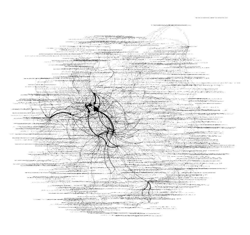
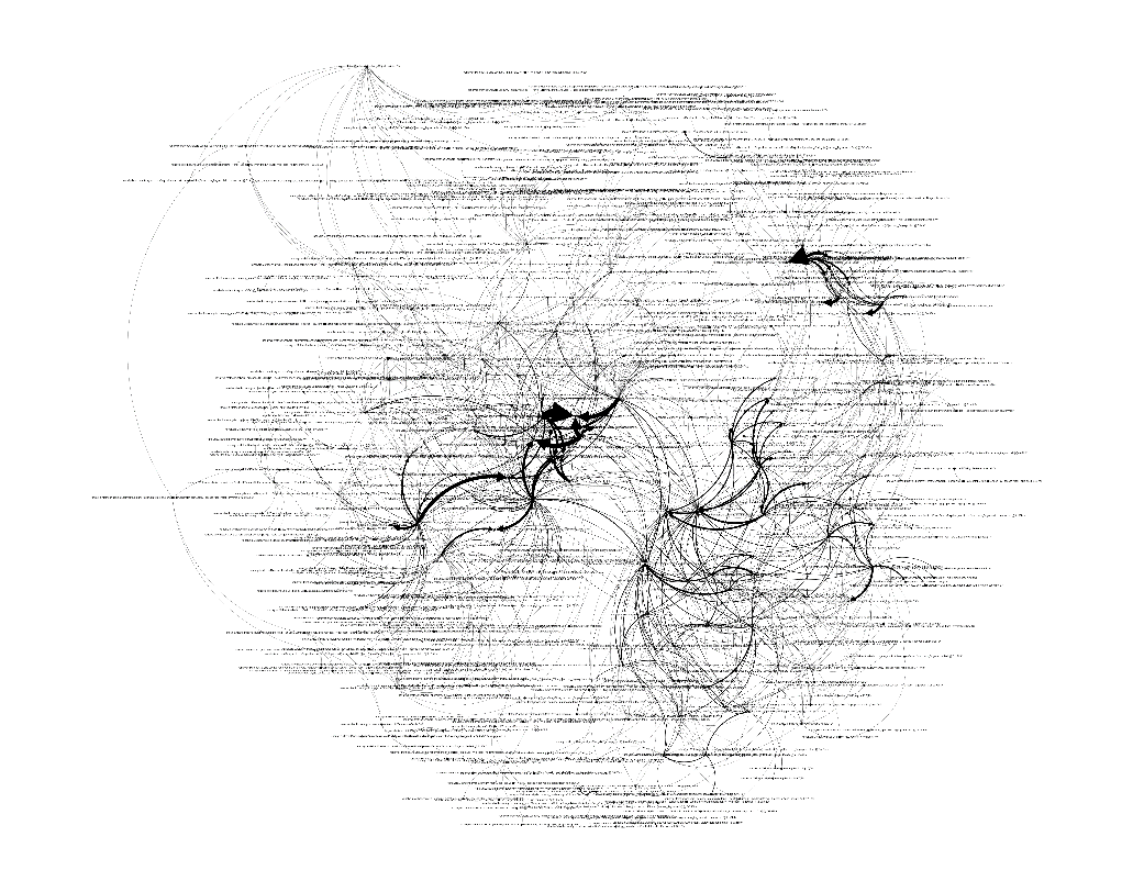
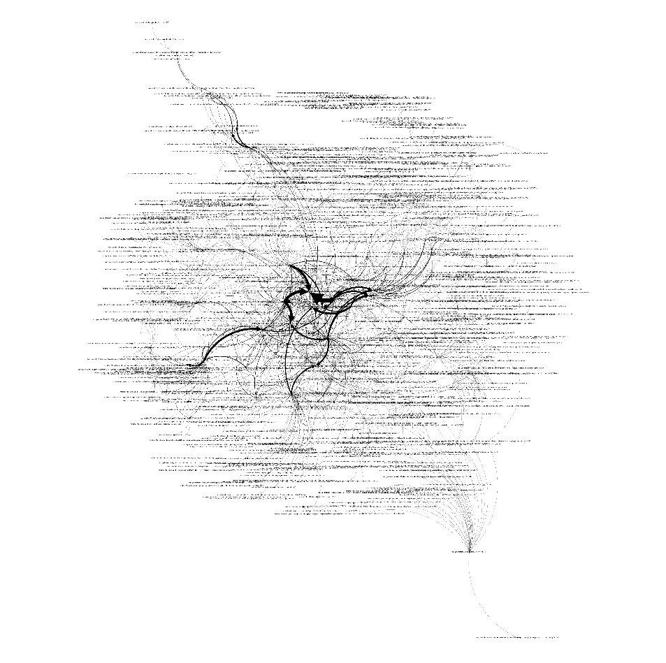
CAGNet converts Android call graphs into fully node-labeled Force Atlas 2 layouts, renders them as greyscale images, and lets a Convolutional Neural Network read the structural behaviour of an app. Explore every stage below — live.
Recreation of Fig. 1 from the paper. Click any stage to see what happens inside it.
A running Force-Atlas-2-style simulation (repulsion + edge attraction + strong gravity, degree-weighted, like the paper's configuration). Pick an app class and watch its call graph self-organize. Hover nodes for full labels — the "full node labelling" that preserves semantics for the CNN. Red nodes mark sensitive / high-risk APIs.


The layout is rasterised to a 250×250 greyscale image — node attributes and structure become pixel values. This is exactly the tensor shape the CNN consumes: (250, 250, 1). Hover the right image to inspect pixel intensities.
Force Atlas 2 call graph (current lab sample)
CNN input — 250×250×1 greyscale tensor
Table III of the paper. Click a layer for its role. Then run the simulated forward pass on the current graph-lab sample — the output mirrors CAGNet's softmax: benign vs malicious probability. (Demonstration only — probabilities are derived from the sample's class, not from the trained model.)
Table IV / Figs. 3–4 of the paper: training samples varied from 600 to the full 8,000. Larger datasets → richer patterns → higher accuracy and lower loss.
| Dataset size | Accuracy (runs) | Loss (runs) |
|---|---|---|
| 600 | 78.67 – 80.25% | 0.751 – 1.013 |
| 2,000 | 84.33 – 86.01% | 0.040 – 0.060 |
| 4,000 | 90.05 – 91.12% | 0.021 – 0.026 |
| 8,000 (CAGNet) | 94.36 – 95.89% | 0.027 – 0.030 |
Chart plots the best run per size. Published charts: Fig. 3 accuracy · Fig. 4 loss.
Table V of the paper — CAGNet is competitive with approaches trained on up to 28,849 samples while using only 8,000.
| Study | Year | Dataset (mal/ben) | Representation | Graph | Classifier | Acc. |
|---|---|---|---|---|---|---|
| [30] | 2024 | 9,998 / 18,851 | uniform feature space | — | SVM, KNN, NB | 97.83% |
| [31] | 2024 | 1,260 / 2,539 | 2D greyscale image | — | CNN | 98.75% |
| [32] | 2023 | 6,368 / 6,530 | GCN vector | FCG | GNN | 94.00% |
| [11] | 2023 | 9,443 / 9,185 | embedded opcode seq. | ICG | Bi-LSTM + GNN | 95.00% |
| [33] | 2022 | 5,560 / 12,686 | GCN vector | FCG | GNN | 95.00% |
| [20] | 2021 | 17,906 / 4,460 | adjacency matrix | CG | CNN | 94.33% |
| [34] | 2020 | 2,130 / 720 | GCN vector | CG | GCN | 92.30% |
| CAGNet | 2025 | 4,000 / 4,000 | node-to-node call graph → FA2 greyscale image | Call graph | CNN | 95.89% |
| Ref | Platform | Graph type | Feature representation | Classifier |
|---|---|---|---|---|
| [15] | Android | ACG | Node2Vec | CNN + DNN |
| [6] | Android | ACG | Word2Vec | CNN |
| [19] | Android | FCG | Bit vector | SVM |
| [20] | Android | ACG | Adjacency matrix | CNN |
| [21] | Android | FCG | Word2Vec | LSTM |
| [17] | Android | GCN | GNN vector | GCN + RNN |
| [22] | Android | DFG | Embedded opcode sequence | GCN |
| [23] | Android | ICG | Node2Vec | LSTM + CNN |
| [24] | Windows | FCG | Adjacency matrix | AEC + CNN |
| [25] | Windows | CFG | GCN vector | GCN |
| [18] | Android | CG | Markov chain | RF, NN, SVM |
| [26] | Android | ICCG | Bit vector | CNN |
| CAGNet | Android | Call graph | Fully labelled FA2 call graph → greyscale image | CNN |
ACG = API Call Graph, FCG = Function Call Graph, GCN = Graph Convolutional Network, CFG = Control Flow Graph, DFG = Data Flow Graph, ICG = Instruction Call Graph, ICCG = Inter-component Call Graph.