CAGNet: Node-Labeled Graph Analysis of Mobile Malware — interactive visualization

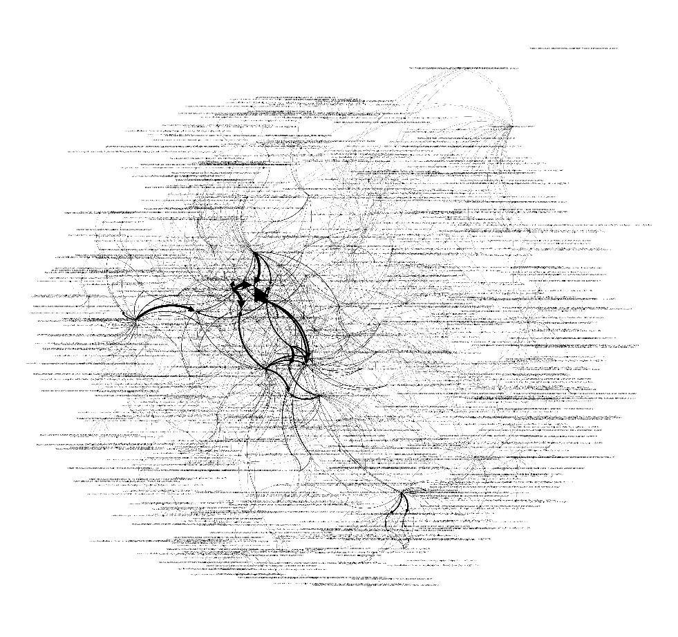
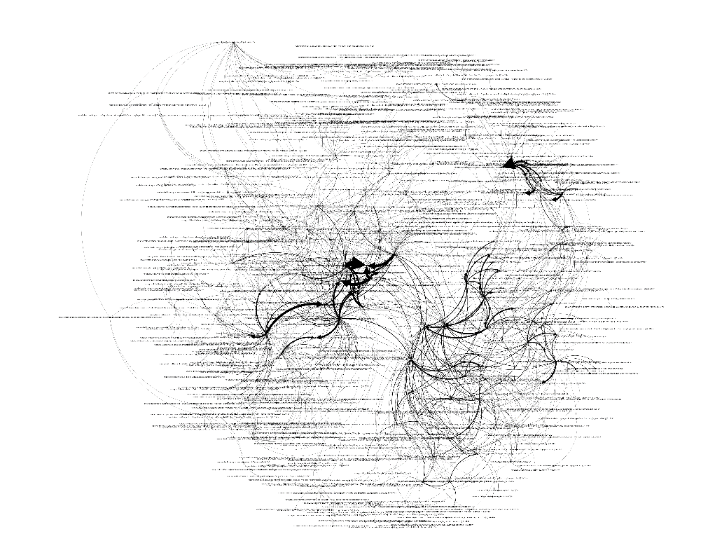
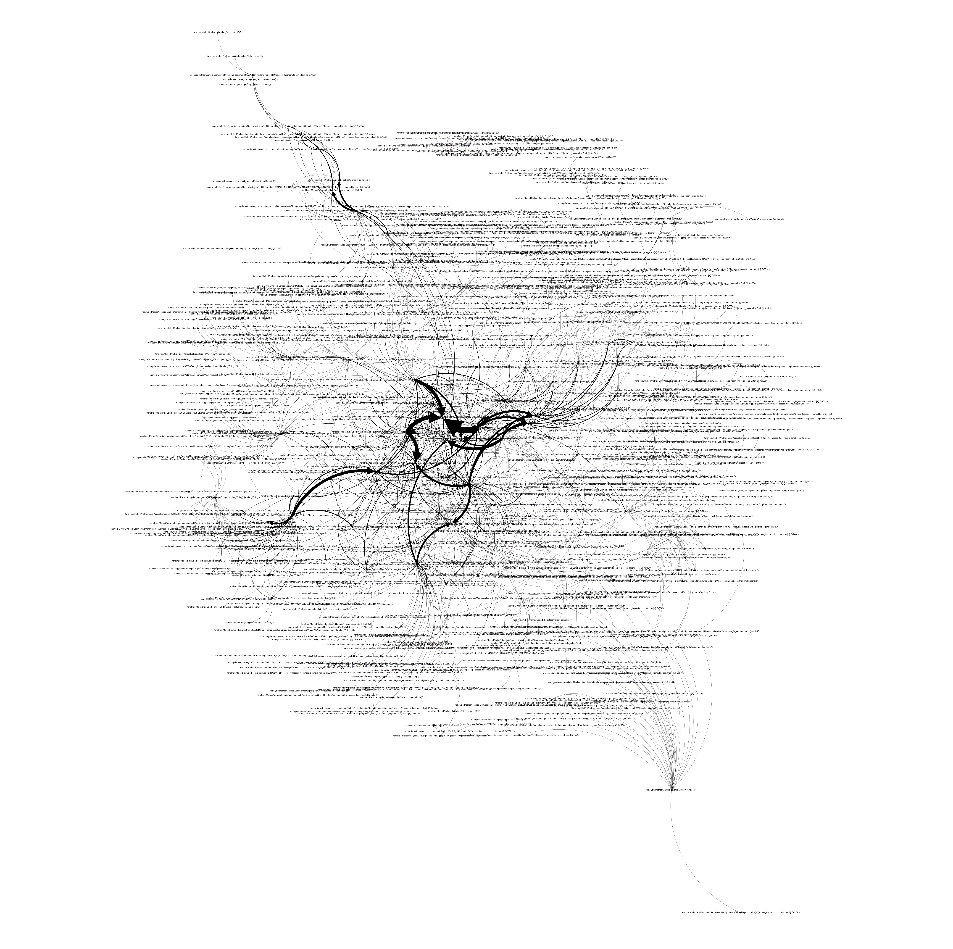
CAGNet converts Android call graphs into fully node-labeled Force Atlas 2 layouts, renders them as greyscale images, and lets a Convolutional Neural Network read the structural behaviour of an app. Explore every stage below — live.

95.89%best detection accuracy (8,000 apps)
8,000APKs — 4,000 malware (AMD) + 4,000 benign (AndroZoo)
250×250greyscale call-graph images fed to the CNN
~1 mintrain/test per run (100 epochs, RTX 3070 Ti)

Stage 1 of the frameworkThe CAGNet pipeline

Recreation of Fig. 1 from the paper. Click any stage to see what happens inside it.

Live demoForce Atlas 2 graph lab LIVE

A running Force-Atlas-2-style simulation (repulsion + edge attraction + strong gravity, degree-weighted, like the paper's configuration). Pick an app class and watch its call graph self-organize. Hover nodes for full labels — the "full node labelling" that preserves semantics for the CNN. Red nodes mark sensitive / high-risk APIs.

Feature representationGraph → greyscale image (250×250)

The layout is rasterised to a 250×250 greyscale image — node attributes and structure become pixel values. This is exactly the tensor shape the CNN consumes: (250, 250, 1). Hover the right image to inspect pixel intensities.

Force Atlas 2 call graph (current lab sample)

CNN input — 250×250×1 greyscale tensor

Deep learning classificationCNN architecture explorer

Table III of the paper. Click a layer for its role. Then run the simulated forward pass on the current graph-lab sample — the output mirrors CAGNet's softmax: benign vs malicious probability. (Demonstration only — probabilities are derived from the sample's class, not from the trained model.)

BENIGN—
MALICIOUS—

Experimental evaluationAccuracy & loss vs dataset size

Table IV / Figs. 3–4 of the paper: training samples varied from 600 to the full 8,000. Larger datasets → richer patterns → higher accuracy and lower loss.

Dataset sizeAccuracy (runs)Loss (runs)
60078.67 – 80.25%0.751 – 1.013
2,00084.33 – 86.01%0.040 – 0.060
4,00090.05 – 91.12%0.021 – 0.026
8,000 (CAGNet)94.36 – 95.89%0.027 – 0.030

Chart plots the best run per size. Published charts: Fig. 3 accuracy · Fig. 4 loss.

State of the artBenchmark comparison

Table V of the paper — CAGNet is competitive with approaches trained on up to 28,849 samples while using only 8,000.

StudyYearDataset (mal/ben)RepresentationGraphClassifierAcc.
[30]20249,998 / 18,851uniform feature space—SVM, KNN, NB97.83%
[31]20241,260 / 2,5392D greyscale image—CNN98.75%
[32]20236,368 / 6,530GCN vectorFCGGNN94.00%
[11]20239,443 / 9,185embedded opcode seq.ICGBi-LSTM + GNN95.00%
[33]20225,560 / 12,686GCN vectorFCGGNN95.00%
[20]202117,906 / 4,460adjacency matrixCGCNN94.33%
[34]20202,130 / 720GCN vectorCGGCN92.30%
CAGNet20254,000 / 4,000node-to-node call graph → FA2 greyscale imageCall graphCNN95.89%

Graph-based classification landscape (Table I)

RefPlatformGraph typeFeature representationClassifier
[15]AndroidACGNode2VecCNN + DNN
[6]AndroidACGWord2VecCNN
[19]AndroidFCGBit vectorSVM
[20]AndroidACGAdjacency matrixCNN
[21]AndroidFCGWord2VecLSTM
[17]AndroidGCNGNN vectorGCN + RNN
[22]AndroidDFGEmbedded opcode sequenceGCN
[23]AndroidICGNode2VecLSTM + CNN
[24]WindowsFCGAdjacency matrixAEC + CNN
[25]WindowsCFGGCN vectorGCN
[18]AndroidCGMarkov chainRF, NN, SVM
[26]AndroidICCGBit vectorCNN
CAGNetAndroidCall graphFully labelled FA2 call graph → greyscale imageCNN

ACG = API Call Graph, FCG = Function Call Graph, GCN = Graph Convolutional Network, CFG = Control Flow Graph, DFG = Data Flow Graph, ICG = Instruction Call Graph, ICCG = Inter-component Call Graph.